Chapter 2 Mapping Data
Written by Paul Pickell
You probably already accept that the Earth is “round” and not “flat”. You have probably held and touched a globe at some point in your life. But have you ever wondered how we describe location and measure something as large as the Earth? In this chapter, we will explore fundamental concepts for how we measure the Earth and orient ourselves with coordinate systems.
- Understand the models of Earth’s figure and shape
- Describe different vertical datums and how they are used to reference height
- Understand the difference between cartesian, celestial, geographic, and projected coordinate systems
- Recognize the differences among major types of map projections
- Explore how projected coordinate systems distort and represent the world around us
Key Terms
Antipode, Great Circle, Small Circle, Geodesy, Vertical Datum, Horizontal Datum, Deflection of the Vertical, Ellipsoid, Spheroid, Geoid, Elevation, Orthometric Height, Geoid Height, Geodetic Height, Coordinate System, Celestial Coordinate System, Cartesian Coordinate System, Geographic Coordinate System, Projected Coordinate System, Map Projection, Tissot’s Indicatrix
2.1 Introduction to Geodesy
Geodesy is the fascinating science of measuring the shape, orientation, and gravity of Earth. Naturally, some of the questions that come to mind when thinking about such a grand topic are I thought the shape of Earth is a sphere? and How do we orient ourselves on Earth? and What does gravity have to do with mapping location?
All of these questions stem from need to represent location. For our purposes, location is the position of something relative to something else. In order to actually describe a location on Earth, we first need to know the size and shape of Earth. Some of the first estimations of Earth’s size and shape were made by Eratosthenes, a Greek mathematician from the second and third centuries B.C. Eratosthenes was responsible for many concepts we use in our everyday lives:
- Conceiving the first spherical model of Earth
- The first accurate measure of Earth’s circumference
- Calculating the tilt of Earth’s axis
- Calculating the distance of Earth to the Sun
- Invention of the leap day
Eratosthenes accurately calculated the circumference of Earth by noticing how the Sun shone directly down the bottom of a well in Syene (modern Egypt) at noon on the summer solstice. He later made a second observation at Alexandria at noon on the summer solstice with a pole and noticed a shadow. He measured the angle of the shadow and inferred the circumference of Earth, which was already known to be spherical (Figure 2.1).
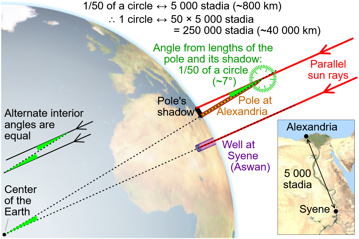
Figure 2.1: Diagram showing how Eratosthenes estimated the circumference of Earth by observing the angle of a shadow that was cast about 800 km north of Syene in present-day Egypt. Monniaux, cmglee, and jimhtatshawdotca (2005), CC-BY-SA-4.0.
Pretty simple, right? Turns out, Eratosthenes was off by only 75 km or less than 0.2% in his calculation! The actual North-South circumference of Earth is about 40,075 km. His calculation worked because the Sun’s rays are nearly parallel when they strike Earth. So if you observe the Sun at the same time in two locations on Earth on the North-South axis, you will notice the Sun has a different elevation above the horizon, which means different lengths of shadows will be cast on the ground. This is also a way to prove that the Earth is in fact round because a flat Earth would have equally-sized shadows everywhere at any given time of day.
2.2 Models of Earth
Here is a simple thought experiment to consider. Suppose you are trying to measure your own height. You probably have not given much thought about how to technically do this because it seems intuitive: place a measuring tape at the bottom of your feet and mark the measurement at the top of your head. If we break this down, there are some important rules to follow (Figure 2.2):
- The measuring tape must originate somewhere. In other words, we need to define a reference point or surface of zero height (i.e., the ground).
- The measuring tape must be a straight line and originate at a 90-degree angle, perpendicular to the ground.
- The measurement must terminate at a point along an imaginary line that is tangential to your head, and yes, that line must be perpendicular to the measuring tape and also parallel with the ground.
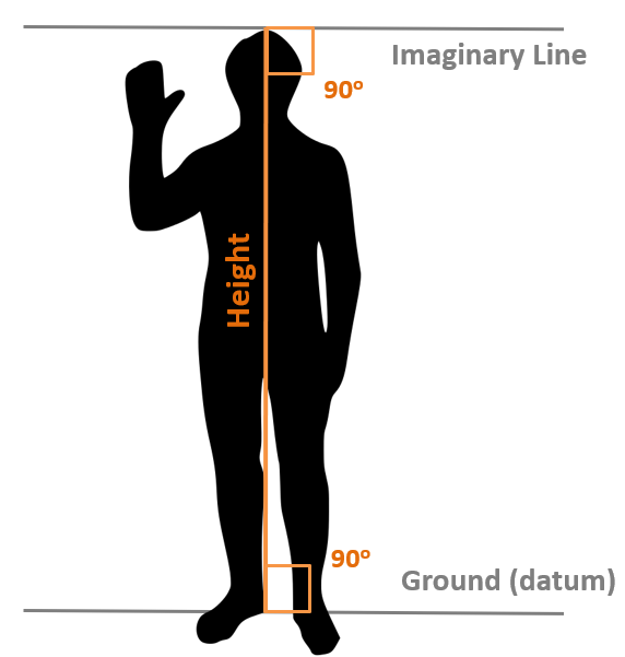
Figure 2.2: Diagram for measuring height above a datum. Pickell, CC-BY-SA-4.0.
Whenever you measure your height, the ground is easy to define. It is whatever point you are standing on. This starting point it also known as a datum. A datum is simply a reference point, set of points, or a surface from which distances can be measured. It does not matter if you are below sea level, atop Mount Everest, or on the 30th floor of a skyscraper. You will always get an accurate and repeatable measure of your height using a datum that is defined directly below your feet. But what about measuring the height of terrain on Earth? Whenever we measure the height of Earth’s terrain above some reference surface, we are measuring elevation.
The same rules above apply when we measure elevation. In order for elevation measurements to be comparable across the world, we need to define a reference surface, a datum, for the entire planet. There are actually several ways that we can model the shape of Earth in order to produce a datum. Models of Earth’s shape are often referred to as either vertical datums (the plural of datum) if you are referencing elevation or horizontal datums if you are referencing location. A vertical datum is a 3D surface model that is used to reference heights or elevations for the Earth. A simple question like How high is Mount Logan in Yukon, Canada? is complicated by the need for a reference surface and the fact that Earth’s shape is irregular. In this section, we will review three types of vertical datums:
- Geodetic - based on geometry
- Tidal - based on sea level
- Gravimetric - based on gravity
2.2.1 Geodetic Vertical Datums
A geodetic vertical datum is one that describes the Earth’s shape in the simplest possible terms using standard geometry. Despite what a globe might lead you to believe, the Earth is not perfectly spherical, but it is close to being spherical. In fact, the radius of Earth varies by no more than 22 km or 0.35%, hardly anything you would ever notice if you were holding it in your hand. That small difference is, however, significant enough to lead to mapping inaccuracies at the local level if a spherical model of Earth was adopted (Figure 2.3). Instead, we frequently describe Earth’s shape as an oblate ellipsoid, which is essentially a sphere that has been flattened, and we define this ellipsoid with a semimajor and semiminor axis. Sometimes you will see the term spheroid used, which just means “sphere-like” and is interchangeable with the term ellipsoid.
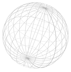
Figure 2.3: Spherical geodetic datum. Pickell, CC-BY-SA-4.0.
There are many different ellipsoids that have been defined and are currently in use as datums. The most commonly used ellipsoid is called the World Geodetic System of 1984 or usually abbreviated as WGS 1984 or WGS 84. In fact, there are hundreds of ellipsoids that have been defined over recent centuries to model the shape of the Earth. The reason for so many other ellipsoids is due in part to technological advances that have improved the accuracy and precision of surveying as well as estimation of the ellipsoidal parameters. Many of these ellipsoids are not geocentric, that is, not originating from the center of mass of Earth. These datums are known as regional datums, which still describe the dimensions that approximate the shape of Earth, but are instead oriented so that the surface of the ellipsoid is congruent with a particular regional surface of Earth. For example, the European Datum 1950, the South American Datum 1969, the North American Datum 1983, and the Australian Geodetic Datum 1966 conform well to their respective continents, even better than WGS 1984 in most cases, but poorly anywhere else in the world.
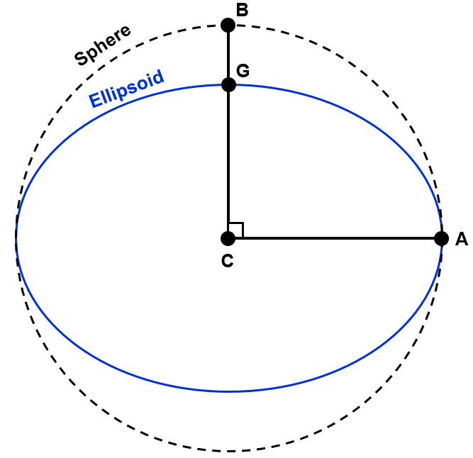
Figure 2.4: Sphere versus ellispoid. Pickell, CC-BY-SA-4.0.
Figure 2.4 greatly exaggerates the flattening of the ellipsoid to illustrate the above points. In reality, the sphere is flattened using a flattening factor calculated as \(f=(CA-CG)/CA\) and defined exactly as \(f=298.257223560\) for WGS 1984. Thus, the semiminor axis (i.e., rotational axis) for the WGS 1984 ellipsoid (meters) is
\[ CG=CA-(CA×\frac{1}{f})=6378137-(6378137×\frac{1}{298.257223560})=6356752.3 \] where \(G\) is the North Pole and \(A\) is a point on the Equator. The sphere, of course, is much simpler where \(radius=CB=CA=6378137\).
2.2.2 Tidal Vertical Datums
A tidal vertical datum is likely one that you are familiar with. The premise of a tidal vertical datum is to use mean sea level as a reference surface, above which are positive elevations and below are negative elevations. This has a lot of advantages, like it is intuitive and oceans cover more than 70% of the planet’s surface so much of Earth’s land mass is near an ocean. However, the disadvantages are that sea level changes over time with tides and also with climate change. The not-so-obvious problem with a tidal vertical datum is that the sea level is actually not constant around the planet not only due to tides, but also temperature, air pressure, and gravity. In other words, mean sea level measured at a gauge station in Halifax on the Atlantic Ocean will not be the same distance from the center of Earth as mean sea level measured at Victoria on the Pacific Ocean (Figure 2.5). The primary challenge with a tidal vertical datum is extending it away from the coastline through a network of survey points using a process known as levelling, and even still, it is only meaningful during the epoch in which the mean sea level was measured at a number of tidal gauge stations.
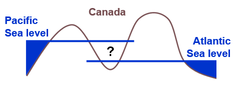
Figure 2.5: Conceptual tidal datum for Canada. Pickell, CC-BY-SA-4.0.
2.2.3 Gravimetric Vertical Datums
The geoid is a physical approximation of the figure of Earth. The shape represents Earth’s surface with calmed oceans in the absence of other influences such as winds and tides. It is computed using gravity measurements of Earth’s surface and is best thought of as the surface or shape that the oceans would take under the influence of Earth’s gravity and rotation alone. In other words, the geoid represents the shape Earth would take if the oceans covered the entire planet. More specifically, the geoid is a gravimetric model of Earth’s shape that is defined as an equipotential surface from a constant gravity potential value. Due to the distribution of mass on Earth, gravity is not constant across the planet’s surface. As a result, the surface of Earth’s oceans is not smooth like a sphere, but instead undulates depending on where gravity forces water to remain at rest. You can think of Earth’s gravitational field as a series of parallel lines extending outwards from the center of mass of Earth into space. Any of these lines that you choose is an equipotential surface where the force of gravity is constant. Keep in mind that the force of gravity is stronger nearer the center of mass of Earth and weaker as you move away from it. Thus, the geoid is an arbitrary equipotential gravity surface that is chosen to roughly coincide with present-day mean sea level.
When you measure the height of something relative to a gravimetric vertical datum like the geoid, you must level your instrument. Levelling forms a vertical line that is orthogonal or perpendicular to the geoid, known as a plumb line. It is incredibly easy to visualize a plumb line. Simply tie a rock to the end of a string and hold the string with your outstretched arm. The length of the straightened string traces a plumb line to the center of mass of Earth, wherever you are. Because gravity changes with location on Earth and all plumb lines are converging on a singular point, plumb lines are never parallel. This phenomenon has important implications for comparing observations on the the ground with a geodetic model of Earth like an ellipsoid. In other words, the plumb line that you traced with your string is pointing to the center of mass of the geoid, but the center of the ellipsoid is often in a slightly different direction. This difference is known as the deflection of the vertical and is measured as the angular difference between the centre of the geoid and the centre of a reference ellipsoid. Like other measurements of geodetic location (i.e., latitude and longitude), the deflection of the vertical is comprised of two angles: \(ξ\) (xi) representing the north-south angular difference and \(η\) (eta) representing the east-west angular difference.
It should be evident by now that the reference surface that you choose as a vertical datum will determine the measured elevation of Earth’s terrain. Additionally, We frequently need to convert elevations between geodetic and gravimetric vertical datums. For example, when you use a Global Navigation Satellite System receiver, you are provided with an elevation that is relative to the WGS 1984 ellipsoid. The difference in height between an ellipsoid and the geoid is referred to as geoid height (N) while the difference in height between an ellipsoid and Earth’s surface is referred to as geodetic or ellipsoidal height (h). The difference in height between the geoid and the Earth’s surface is called orthometric height (H) (Figure 2.6), and is given as:
\[ H = h - N \]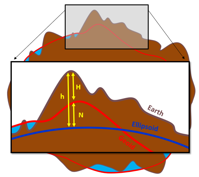
Figure 2.6: Orthometric Height (H) is the ellipsoidal height (h) less the geoid height (N). Pickell, CC-BY-SA-4.0.
To illustrate the concept of a gravimetric datum, suppose we constructed a large, straight tunnel through the physical Earth that was tangential to the ellipsoid. If we allowed the oceans to flow freely through this tunnel, your experiences might convince you that water would flow from one end to the other. But in fact, this tunnel is so large, that the gravity field is changing. So the water would actually come to rest at the surface of the geoid or gravimetric model, as shown in Figure 2.7 below.
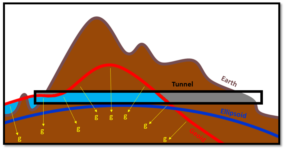
Figure 2.7: Thought experiment showing where water would be at rest within a tunnel through the geoid due to the equipotential force of gravity (g). Pickell, CC-BY-SA-4.0.
2.3 Case Study: The Canadian Geodetic Vertical Datum of 2013
The Canadian Geodetic Vertical Datum of 2013 (CGVD2013) is the current gravimetric vertical datum used in Canada to reference heights. It is defined with a potential gravity value of 62,636,856.0 \(m^2\) \(s^-2\). The pervious vertical datum in Canada - the Canadian Geodetic Vertical Datum of 1928 (CGVD28) - was actually a tidal vertical datum that corresponded to mean sea level measured at Yarmouth, Halifax, Pointe-au-Père, Vancouver and Prince-Rupert, and a height in Rouses Point in New York. It turns out that Halifax referenced to CGVD2013 is 64 centimeters below Halifax referenced to CGVD28!
For reference, CGVD2013 is 17 centimeters below mean sea level measured in Vancouver at the Pacific Ocean, 39 centimeters above mean sea level in Halifax at the Atlantic Ocean, and 36 centimeters above mean sea level in Tuktoyaktuk at the Arctic Ocean. The older CGDV28 did not have any survey benchmarks in the far north of Canada and, with the advent of more reliable satellite-based measurements, was modernized in 2015 to CGVD2013. The United States currently uses the North American Vertical Datum of 1988 (NAVD88), which was never adopted by Canada, but the United States will be modernizing their vertical datum by adopting a gravimetric model with the same gravity potential value as Canada as early as 2025.
Figure 2.8: The difference (in meters) between the Canadian Geodetic Vertical Datum of 2013 (CGVD2013) and the Canadian Geodetic Vertical Datum of 1928 (CGVD28). Animated figure can be viewed in the web browser version of the textbook. Data from Natural Resources Canada and licensed under the Open Government Licence - Canada. Pickell, CC-BY-SA-4.0.
2.4 Referencing Location
2.4.1 Cartesian Coordinate Systems
Now that we have explored how to reference heights to vertical datums, we will now turn to considering how to reference location on Earth. Before we we jump to the three dimensional case of Earth, consider how you would map your room and identify your location within that room. Assuming you are in a rectangular room, you could easily pick a corner and first measure the distances between the four corners of the room, giving you the dimensions. You could then proceed to measure your distance to any two walls and quite easily define your position within the room relative to the first corner that you picked. This is an example of a coordinate system that provides reference for the relative locations of anything contained within the extent of the coordinate system (i.e., the four corners of your room).
Fundamentally, a coordinate system is defined by a common unit of measurement (e.g., meters, feet, degrees), an orientation defining the direction that measurements positive or negative, and an origin, which is an arbitrary point where the measurements begin at zero. On a one dimensional line, you can define any other location on the line as a measured distance from the origin at \([0]\). On two dimensional maps, like your room, we have two axes that are perpendicular from which we can define any location with measured distances from the origin \([0,0]\). We can also extend this to the three dimensional Earth, which simply requires another axis to define the origin at \([0,0,0]\). All of these cases are referred to as Cartesian coordinate systems, so-named after French philosopher Descartes (also known for the phrase, “I think, therefore I am”) who first described the two dimensional case in 1637 in La Géometrie.
2.4.2 Celestial Coordinate Systems
You might be wondering, How do we reference locations on Earth? Before the technological era of geoids, astronomical observations provided the basis for the earliest coordinate systems. The ancient civilizations of Greece, Egypt, and Babylon all recognized the use of celestial coordinate systems for defining the location of stars, planets, and other celestial bodies in the sky. Recall that Eratosthenes, a Greek mathematician living about 2300 years ago, had already worked out the spherical shape of Earth. A celestial coordinate system simply extends the spherical shape of the Earth outward into space to locate objects using angular measurements. It is a geocentric coordinate system, that is based on an origin at the center of Earth with an orientation following the rotational axis of Earth (i.e., spinning around the semiminor, North-South axis). This is also known as an equatorial coordinate system, because it is oriented relative to the Equator of Earth. The equatorial coordinate system is the reason why you can navigate by Polaris, the North Star, which would appear nearly directly overhead if you were standing at the North Pole. Even though Earth is not perfectly spherical, astronomical observations have been reliably used for millennia to transit the irregular oceans and terrain of Earth.
2.4.3 Geographic Coordinate Systems
Geocentric coordinate systems are essential for global navigation and mapping. In the modern era, we use geographic coordinate systems (sometimes abbreviated GCS) that are oriented to the rotational axis of Earth, much like the equatorial coordinate system. The origin of a geographic coordinate system is the center of Earth and the units of measurement are degrees of longitude and degrees of latitude. Degrees of latitude (denoted by lambda, \(λ\)) measure the angle from the equitorial plane North (+) or South (-), while degrees of longitude (denoted by phi, \(φ\)) measure the angle from the polar plane East (+) or West (-). Thus, geographic coordinate systems use angular units of measurement. Any combination of latitude and longitude gives coordinates \([λ,φ]\) on a sphere or ellipsoid. Positive values of latitude put you in the Northern Hemisphere, while negative values of longitude put you in the Western Hemisphere. Constant lines of latitude, known as parallels because they are always parallel to one another, and lines of longitude, known as meridians, form a grid that fits over a sphere or ellipsoid called a graticule.
For most of your life, you have probably believed that there is a singular combination of capital-L Latitude and Longitude values that absolutely define some location on Earth in perpetuity. This is perhaps the most profound geographic lie that we were taught as young school children. In fact, there are as many “types” of latitude as there are geographic coordinate systems. By now, you should be able to recognize the difference between geocentric latitude that is referenced to a sphere and geodetic latitude that is referenced to an ellipsoid. The main difference is that geocentric latitude is the angle relative to the centre of the sphere at the equatorial plane and geodetic latitude is the angle relative to the equatorial plane (i.e., not necessarily the centre). Figure 2.9 illustrates how the same angle can put you in two very different places depending on the geographic coordinate system you are using.
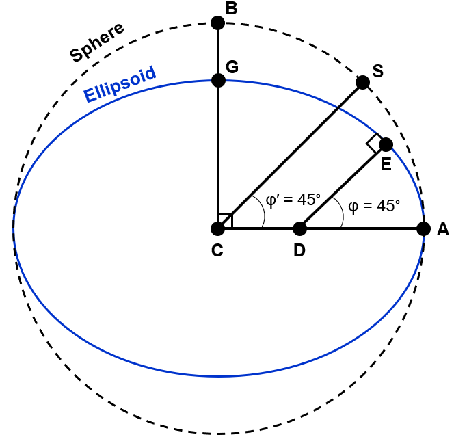
Figure 2.9: Geocentric versus geodetic latitude. Pickell, CC-BY-SA-4.0.
\(CS\) represents the line connecting the centre of a spherical geographic coordinate system to the surface of the sphere at a geocentric latitude \(φ′=45°\) and \(DE\) represents the line connecting the equatorial plane to the surface of the ellipsoid at a geodetic latitude \(φ=45°\). Notably, \(CS\) is parallel to \(DE\) and \(CS\) intersects with the surface of the sphere at a 90° angle and \(DE\) intersects the surface of the ellipsoid at a 90° angle.
A coordinate system that is referenced to an ellipsoid is known as a horizontal datum. For example, the World Geodetic System of 1984 (WGS 1984) is a geodetic datum that has a geographic coordinate system referenced to it. So the origin of WGS 1984 is also the origin of the GCS from which latitude and longitude measurements are derived. So if you measured your latitude and longitude using the WGS 1984 horizontal datum, you would be placed somewhere on the ellipsoid also defined by WGS 1984. It is important to note, however, that the same exact geocentric latitude and longitude measures would place you somewhere else on a sphere. Other factors such as plate tectonics, glaciation, and ocean tides cause the Earth’s surface to be in constant motion underneath any fixed horizontal datum. For example, Europe has drifted about 60 meters from North America since Eratosthenes first calculated the circumference of Earth. Therefore, any “type” of latitude or longitude is only useful during a particular epoch of time.
If you mapped the Earth as an ellipsoid in a three dimensional Cartesian coordinate system, you could describe location using three coordinates \([x,y,z]\), with \([0,0,0]\) being the center of Earth. However, we do not often express mapped coordinates of Earth using Cartesian coordinates. Instead of referring to the North Pole at \([0,0,6356752.3]\) meters (the polar radius of Earth) we usually refer to it with a single coordinate, 90° N. Why? The North and South Poles are the only points on Earth that can be defined with a single coordinate because they coincide with the orientation of a geographic coordinate system. Imagine placing a protractor at a 90° angle relative to a table. If you rotate it along that perpendicular axis, one arm of the protector would spin in a 360° circle, but the other arm of the protractor would always point up or down at 90° in the same direction. For all other locations on Earth, a pair of \([λ,φ]\) coordinates are needed to define location. With space-based global navigation systems it is more common to combine coordinates in both horizontal and vertical datums together. For example, \([λ,φ]\) expresses your location relative to the horizontal datum while \([λ,φ,h]\) expresses your ellipsoidal height (h) at a location and \([λ,φ,H]\) expresses your orthometric height (H) at a location.
Your Turn!
Use our geodesy tool to visualize the differences between the sphere, ellipsoid, and geoid. You can modify the transparency of the sphere and ellipsoid to see how these geometries vary. Change the flattening of the ellipsoid to achieve different models of Earth. Search for locations with latitude and longitude values and calculate the geoid height. Compare geocentric and geodetic latitudes. The sphere and the ellipsoid models in the visualization represent Earth’s equatorial diameter (semi-major axis) as 6,356,752.3 m (i.e., equivalent to WGS 1984) and the geoid elevations are exaggerated by a factor of 0.549 to enhance their appearance.
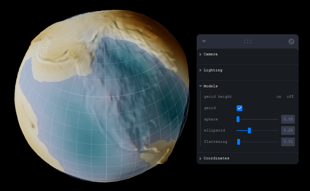
Figure 2.10: Online geodesy tool for visualizing the differences between the sphere, ellipsoid, and geoid. Click here to access the interactive tool. Floria Gu, CC-BY-SA-4.0.
2.4.4 Projected Coordinate Systems
Despite everything covered so far in this chapter, we very rarely see or display geographic data in 3-dimensions. In fact, most geographic data you will likely encounter will be either 1- or 2-dimensional. Geographic coordinate systems are incredibly important for understanding how geographic data are fundamentally “attached” to the Earth. However, geographic coordinate systems are not suitable for creating maps, those 2-dimensional spatial models that can be easily displayed on your computer screen or printed on a sheet of paper. Instead, cartographers rely on projected coordinate systems that flatten a 3-dimensional geographic coordinate system to a 2-dimensional map. Really, these projected coordinate systems involve transformations called map projections that convert 3-dimensional coordinate space into 2-dimensional coordinate space, which means the map units are linear such as meters. Whenever we move from a geographic to a projected coordinate system, we lose information, and distortion results.
Cartographers have wrestled with how to project Earth onto a printed page for millennia. The fundamental mathematics for map projections were first comprehensively described by Claudius Ptolemy around 150 C.E. Ptolemy’s work Geography was one of the earliest treatises on cartography and map making that included an atlas of regional maps of Europe, Africa, and Asia. Ptolemy’s work built on and came several centuries following Eratosthenes and earlier Greek geocentric observations by Plato and Aristotle. Ptolemy observed that a globe was the best way to represent the intervals and proportions of Earth’s surface without distortion. However, globes are not very useful for looking at regions in detail and you can only see part of a globe at any given time. Thus, a mathematical language is needed to translate a geographic coordinate system to a planar or projected coordinate system. Geography was lost to antiquity before it was rediscovered, copied, and translated centuries later, first by Muslim cartographers in the 9th century C.E. and later by Italian cartographers in the 15th century C.E. during the Renaissance, which gave rise to the many types of map projections that we see today.
Because all map projections result in distortion from the loss of the third spatial dimension, it is useful to think about map projections in terms of what they preserve. There are four main characteristics that can be distorted or preserved, which give rise to the primary types of map projections that are in use for environmental management applications:
- Conformal projections preserve shape and angles
- Equal-area or equivalent projections preserve area
- Azimuthal projections preserve direction
- Equidistant projections preserve scale and distances
Some map projections can preserve several of these characteristics at once, but only a globe can simultaneously preserve area, direction, distance, and shape. Any map projection will have inherent trade-offs representing these characteristics accurately. It is beyond the scope of this textbook to discuss all map projections. Instead, we will focus on several key examples of map projections that are commonly used for environmental management applications. For a more comprehensive discussion of map projections generally, the reader is referred to Map Projections: A Working Manual by (Snyder 1987). In the next section, we look at how map projection distortation can be measured.
2.4.5 Measuring Map Projection Distortion
Tissot’s Indicatrix is often used to visualize distortion from map projections, named after Nicholas Auguste Tissot. The metric is relatively simple: Tissot’s Indicatrix is a perfect circle on the surface of a 3-dimensional globe, but will form an ellipse whenever projected to a 2-dimensional coordinate system. For this reason, Tissot’s Indicatrix is sometimes referred to as Tissot’s Ellipse. Since ellipses can vary along two axes, Tissot’s Indicatrix can represent areal, angular, and linear map distortions both longitudinally and latitudinally at any location in the map. This is very handy, because we can place Tissot’s Indiciatrices (the plural of indicatrix) at different locations and examine how distortion changes throughout the map projection.
So how do we use this tool? The quotient between a line projected onto a map \(a\) and the same line on a globe \(a'\) is \(\frac{a}{a'}=1\) when there is no distortion on that axis of the ellipse. This quotient is also called a scale factor because it is showing how the map scale is modified locally by a map projection. Figure 2.11 below shows an example of a reference indicatrix that is a perfect circle on a globe with axes \(a\) and \(b\).
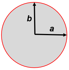
Figure 2.11: Reference Tissot Indicatrix. Pickell, CC-BY-SA-4.0.
Let us assume that \(a = b = 1\). Then, the reference indicatrix has the following properties: \(a=b\), \(a×b=1\), and \(Area=πab=π\). If \(\frac{a'}{a'}>1\), then we can conclude that the the projection is expanding the distance along the \(a\) line. If \(\frac{a'}{a'}<1\), then we can conclude that the projection is compressing the distance along the line \(a\). For example, suppose \(a=2\) and \(b=0.5\), then we have modified the scale of the indicatrix along both axes, but the areal solution is the same as the reference indicatrix shown as the red dashed circle in Figure 2.12 below.
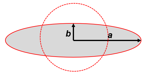
Figure 2.12: Equivalent Tissot Indicatrix. Pickell, CC-BY-SA-4.0.
The indicatrix above in Figure 2.12 is an example of an equivalent indicatrix, which has the following properties: \(a>b\), \(a×b=1\), and \(Area=πab=π\).
If \(\frac{a}{a'}×\frac{b}{b'}>1\), then we can conclude that the projection is inflating the area. If \(\frac{a}{a'}×\frac{b}{b'}<1\), then we can conclude that the projection is deflating the area. Consequently, whenever the quotients of both axes are equivalent (i.e., \(\frac{a}{a'}=\frac{b}{b'}\)), Tissot’s Indicatrix forms a perfect circle and the ellipse is conformal with angles true to the globe. For example, suppose \(a=b=2\), then we have modified the scale of the indicatrix along both axes, but with the same factor. This results in a conformal indicatrix that is not equivalent, shown in Figure 2.13 below.
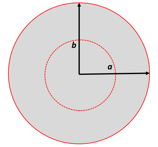
Figure 2.13: Conformal Tissot Indicatrix. Pickell, CC-BY-SA-4.0.
This conformal indicatrix has the following properties: \(a=b\), but \(a×b≠1\), and therefore \(Area=πab=4π\). As you can see, whenever \(a×b=1\) the indicatrix is equivalent (equal-area) and whenever \(a=b\) the indicatrix is conformal.
2.5 Map Projections for Environmental Management
2.5.1 Mercator
Mercator is a cylindrical map projection that represents meridians and parallels as straight lines. The cylindrical surface is oriented such that the rotational axis of Earth runs through the openings of the cylinder and the Equator represents the tangent where the cylinder meets the Earth’s surface. Scale along the tangent is true because the translation from the spherical Earth to the cylindrical surface is one-to-one at the tangent, so this is also the location on the projection where there is no distortion. This has the effect of accurately representing the shape and angles on the map (i.e., conformal), but greatly distorts area as you move away from the Equator. In fact, the North and South Poles are represented as 2-dimensional lines at the top and bottom edges of the map instead of 1-dimensional points. Although scale and area change as you move North or South along a meridian, scale and area are equivalent along any parallel, but not necessarily true to a globe. In other words, you can compare area or scale anywhere along a parallel, but only at the Equator is the area and scale true to the globe.
The Mercator map projection is perhaps the most pervasive and reproduced projection around us (Figure 2.14). Because angles are preserved, you can easily and accurately navigate long distances across Earth, and this was exactly the purpose that Gerardus Mercator envisioned when he first identified the projection for sea-faring Europeans in 1569. You may also recognize the Mercator projection from web mapping applications like Google Maps, which use it because it ensures that North-South roads intersect at right angles with East-West roads.
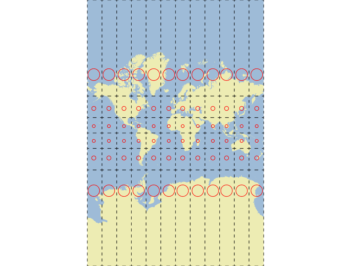
Figure 2.14: Mercator map projection with Tissot’s Indicatrices in red. Pickell, CC-BY-SA-4.0.
2.5.2 Universal Transverse Mercator (UTM)
Universal Transverse Mercator (UTM) is very similar to a Mercator projection except that the cylinder is rotated or transverse by 90° so that the opening of the cylinder is perpendicular to the rotational axis of Earth. This has the effect of moving the tangent from the Equator to any Meridian. In fact, you can rotate the cylinder at any angle you want where 0° is a true Mercator, 90° is a transverse Mercator, and any other angle is considered an oblique Mercator. UTM is actually a system of 60 different transverse Mercator projections that are defined to represent 6° Longitudinal intervals of Earth’s surface (60 zones x 6° = 360°). Each projection is defined as a zone, which is also divided into North and South zones depending whether you are in the Northern or Southern Hemisphere. Canada spans 16 UTM zones from Zone 7 North in the Yukon to Zone 22 North covering Newfoundland. Figure 2.15 below shows a map of UTM Zone 13 over Saskatchewan.
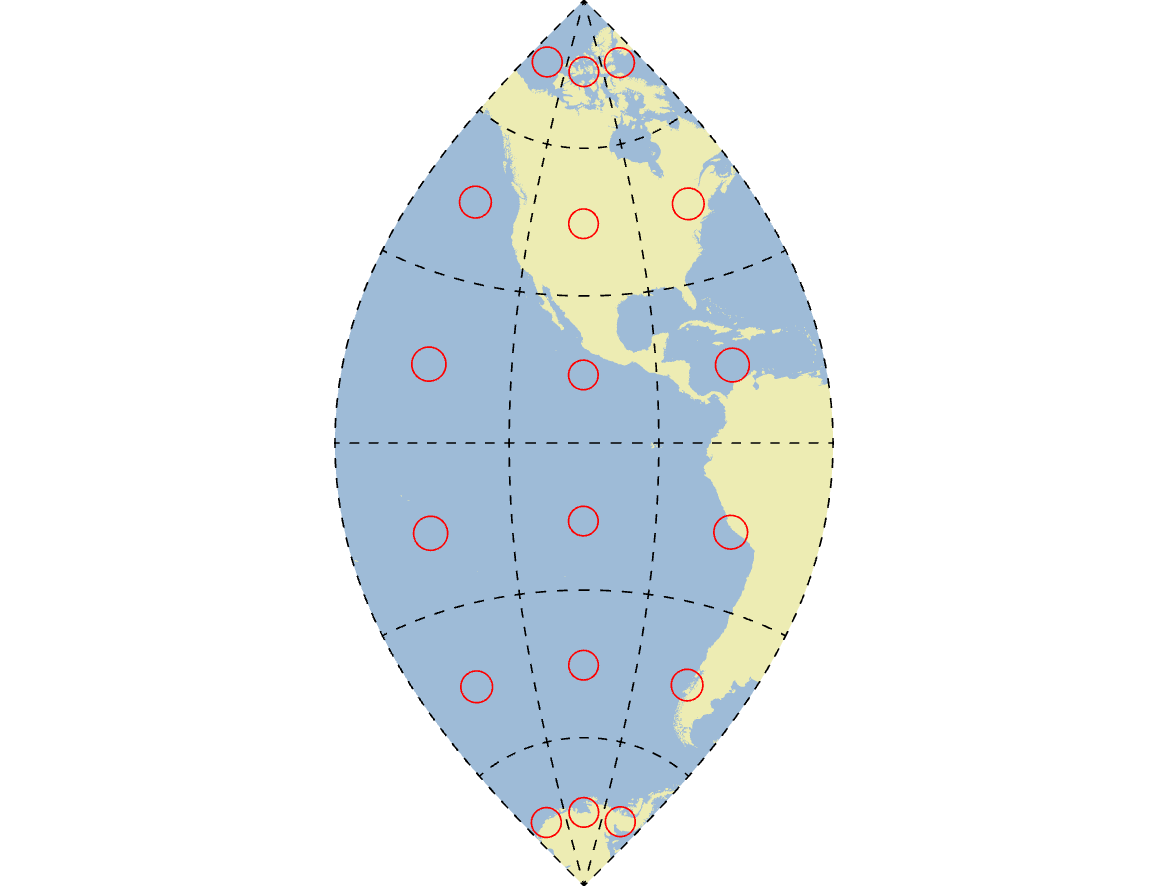
Figure 2.15: Universal Transverse Mercator Zone 13 map projection with Tissot’s Indicatrices in red. Pickell, CC-BY-SA-4.0.
Besides defining the orientation of the cylinder, we can also specify its size or diameter. When the diameter of the cylinder is equivalent to the diameter of Earth at the Equator, a single tangent line is formed. If the diameter of the cylinder is smaller than Earth’s diameter at the Equator, then the cylinder has two lines that contact Earth’s surface, known as secants. The purpose for having two secants is that the projection distortion can be more evenly distributed across the map. In the case of UTM, a scale factor of 0.9996 is applied to shrink the transverse cylinder slightly, forming two secants that are 360 km apart East-West. In between the two secants lies the central meridian, which is used to define the origin for the projected coordinate system. It is important to realize that the secants are parallel to each other and the central meridian, which means the secants are not meridians on Earth and form what are called small circles, a line that does not divide Earth into two equal portions.
UTM uses a unique coordinate system that deserves some explanation. Just like with latitude and longitude coordinates \([λ,φ]\), an arbitrary origin needs to be defined so that we know where we are in relation to the origin on the map. For projected coordinate systems like UTM that use linear units of measure such as meters, the origin is defined as the intersection of the central meridian and the Equator. Simple enough, right? There is one catch: UTM does not use any negative coordinates by convention. Thus, the origin of the coordinate system for each zone must be moved so that coordinates West of the central meridian and South of the Equator are positive. To do this, a constant value is added to all East-West coordinates (known as Eastings) and all North-South coordinates (known as Northings) to create what are known as False Eastings and False Northings, respectively. A value of 500,000 m is added to all Eastings so that the western limit of the zone is located at 0 m, the central meridian is located at 500,000 m, and the eastern limit of the zone is located at 1,000,000 m. A value of 10,000,000 m is added to all Northings in the Southern Hemisphere so that the Equator is at 10,000,000 m and 0 m is near the South Pole for all southern UTM zones. You might recognize the importance of the 10,000,000 m value because this represents approximately one-quarter of the Earth’s North-South circumference.
2.5.3 Sinusoidal
Sinusoidal is a pseudocylindrical map projection, so-named because these projections approximate a true cylindrical projection except that Meridians are curved instead of straight like with Mercator or UTM. Because Meridians are curved, Sinusoidal maps represent the North and South Poles as single points instead of lines as is the case with Mercator. Thus, Sinusoidal maps are not conformal and distort shape, but they are in fact equal-area (Figure 2.16). Equal-area map projections like Sinusoidal are important for accurately accounting for land cover and other global mapping efforts. Therefore, it is common to find global datasets distributed in a Sinusoidal map projection.
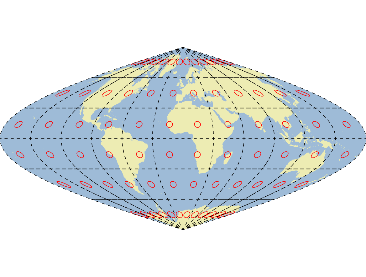
Figure 2.16: Sinusoidal map projection with Tissot’s Indicatrices in red. Pickell, CC-BY-SA-4.0.
2.5.4 Albers
Albers is another example of an equivalent map projection, but unlike Sinusoidal, an Albers projection uses a cone as a projection surface instead of a pseudocylinder. Like the cylindrical case, the cone can be sized and oriented in any way, but the cone of an Albers projection is typically oriented so that the vertex of the cone aligns with the rotational axis of Earth. The base of the cone has a diameter that usually results in two secants, known as standard parallels on an Albers map. Thus, Albers projections tend to distort latitudinally as you move North-South away from the standard parallels, but even more so as you move toward the base of the cone (Figure 2.17). Besides being an equal-area projection, Albers is a good choice for mapping regions because shape and scale are mostly preserved near the standard parallels. For example, the province of British Columbia has adopted a modified Albers projection that situates the standard parallels at 50° N and 58.5° N, which are near the northern and southern latitudinal limits of the province. This narrow band of latitude between the standard parallels ensures that there is relatively little distortion in shape and scale within the province, which is comparable to UTM. However, British Columbia is a longitudinally wide province, spanning 6 of Canada’s 15 total UTM zones, so Albers has a distinct advantage of being able to show the entire province with little distortion. For the same reasons, you will often find Canada-wide data distributed in an Albers projection.
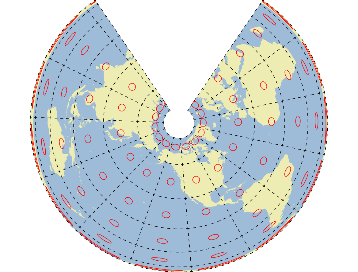
Figure 2.17: British Columbia Environment Albers map projection with Tissot’s Indicatrices in red. Pickell, CC-BY-SA-4.0.
2.5.5 Azimuthal
Azimuthal projections use a flat circular plane to project the Earth onto a map. This plane is usually oriented so that it is tangent at a single point, usually the North or South Pole. In the case of a polar azimuthal projection, meridians radiate outward as straight lines from the pole to the edge of the circular plane and the parallels are represented as concentric circles. As a result, distortion increases as you move away from the centre point of the map with the outer edge of the plane representing an antipode or an opposite point on Earth. The primary benefit of azimuthal projections is that they preserve direction and distance between the centre point and any other point in the map (Figure 2.18). The shortest geographic distance between the centre point and any other point creates a line known as a great circle, which divides the Earth into two equal portions. So another benefit of an Azimuthal project is that great circles can be mapped as straight lines. Azimuthal projections are commonly used when distance and direction are important, such as weather RADAR stations or air traffic control towers. It is important to realize that the centre point for an azimuthal projection can be any point on Earth and the equidistant property can be exploited for a number of applications.
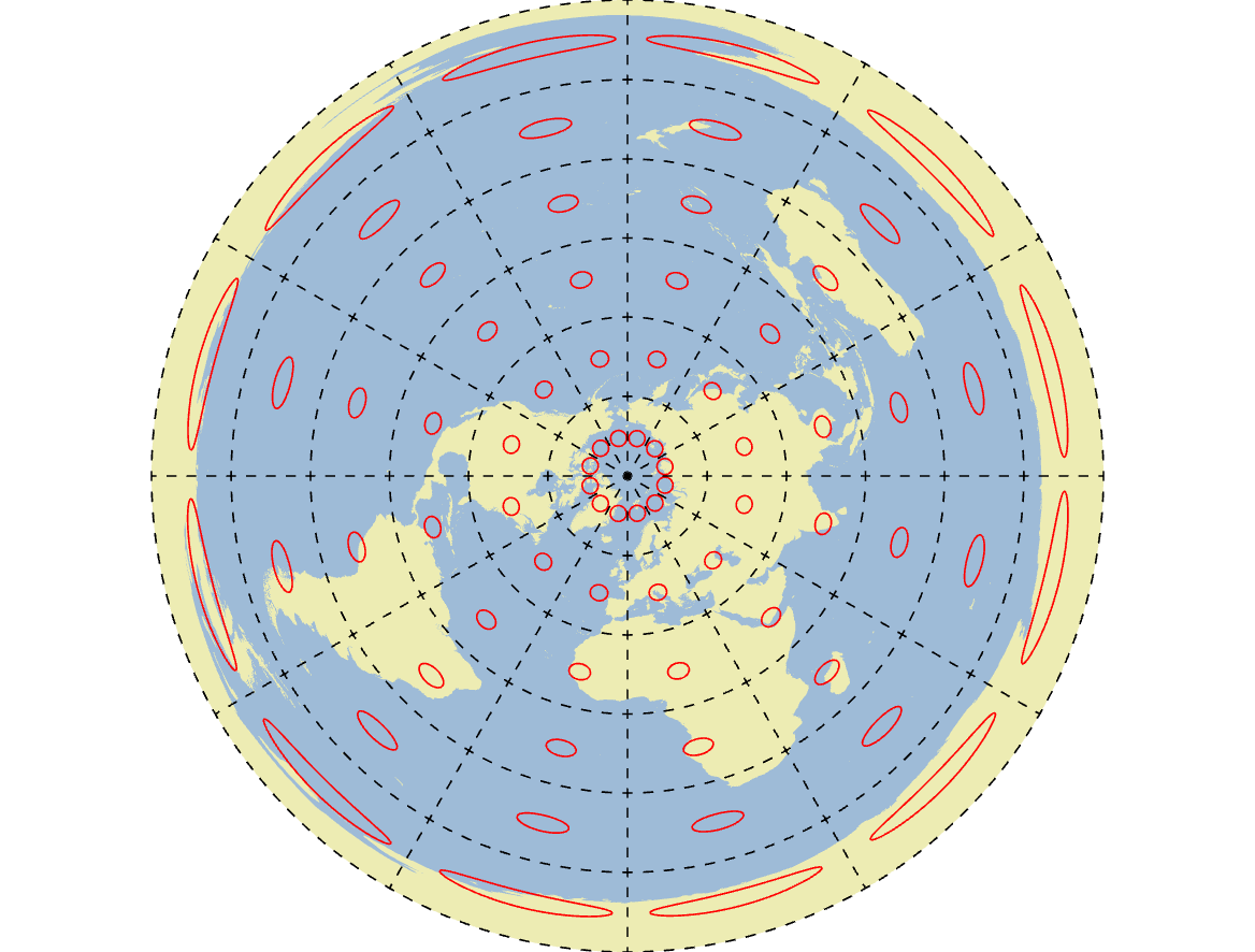
Figure 2.18: North Pole Azimuthal map projection with Tissot’s Indicatrices in red. Pickell, CC-BY-SA-4.0.
2.6 Summary
In this chapter, you learned about the science and technology of geodesy that goes into mapping data. We described the different models of Earth’s shape and the advantages and disadvantages that each model has. More generally, models of Earth represent vertical datums to which heights are referenced. When we think of “where” something is on Earth, we must use horizontal datums to reference location. There are two types of horizontal datums that are very important to geomatics: (1) a geographic coordinate system uses lines of latitude and longitude to define locations on Earth’s 3-dimensional surface while (2) a projected coordinate system flattens Earth into a manageable 2-dimensional coordinate space. In the case of projected coordinate systems, we have many choices when deciding which map projection to use when we map data, each with its own uses and distortions. The next time that you look at a map, ask yourself with your new found appreciation of geodesy, how is this information being misrepresented to me?